
Actuarial reserve valuations are computationally intensive, often requiring hours or even days to complete a large valuation run. However, for many ad hoc analyses, speed is more critical than precision. This is when having a lightweight but robust proxy model becomes useful. A good proxy model should have the following properties: 1) given the same inputs, it produces reserves similar to those from the full valuation model, and 2) it is computationally easy (e.g., relying on closed-form formulas). This article discusses the theory and practice behind creating such a proxy model.
Theory
Neural networks have become the predominant algorithm in the field of artificial intelligence, underpinning many of the most powerful models in natural language processing, computer vision, and numerous other real-world applications.[1] It turns out that neural networks are also excellent candidates for proxy models! This claim is founded on the Universal Approximation Theorem, which states that any function can be approximated arbitrarily closely by a neural network. Simply put, if you build a neural network to approximate a reserve function and are not satisfied with the result, you can continually tweak or increase the size of the network to bring the neural network outputs closer and closer to the actual reserves.
Another reason neural network is a good candidate for proxy model is that, despite its complexity, a trained neural network is computationally easy. It involves only basic matrix multiplications and simple activation functions—all of which are elementary mathematical operations that a computer can perform quickly and easily. (See Figure 1)
Figure 1
How a Neural Network Functions
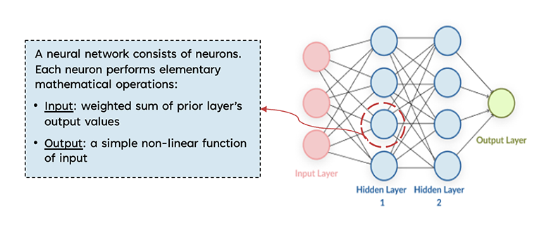
We can use supervised learning techniques to train the neural network, feeding the model many examples of valuation input-output pairs. The neural network learns to “predict” reserve by iteratively adjusting its model parameters (or “weights”) to minimize the difference between predicted and actual reserves. Once trained, the model can approximate reserve for any policy and input values going forward.
Experiment
In this section, we discuss a case study where we trained a neural network to compute Variable Annuity Guaranteed Lifetime Withdrawal Benefits (VA GLWB) fair value reserves. VA GLWBs were chosen because reserve calculations for these products are notoriously complex. They are essentially exotic options, and when layered with dynamic policyholder behavior assumptions, the math becomes intractable. Monte Carlo simulations are the only practical method to value these benefits, but they are very time-consuming.
Our first step was to generate a large dataset of valuation input-output pairs using a full valuation model. Inputs included policy attributes and economic variables such as interest rates and equity volatilities. To ensure a good fit, we generated a wide range of values for these inputs. The outputs were the corresponding seriatim reserves (based on 250 risk-neutral scenarios) from the full valuation model. In total, 250,000 data points were generated. To make the case study realistic, our VA GLWB product included typical features seen in the marketplace (e.g., ratchets), as well as a dynamic lapse assumption.
Next, we constructed a fully connected neural network[2] with three hidden layers and used 60% of the generated input-output pairs to train the model. This training was the most time-consuming step, but it is a one-time effort. The trained neural network would remain a reasonable proxy for the full valuation model as long as there are no significant changes to the latter.
After training, we evaluated the model on the remaining 40% of the data. As shown in Tables 1 and 2 below, the results from the proxy model were very close to those from the valuation model, both in aggregate (0.2% difference) and at the seriatim level.
Table 1
Full Results on 100,000 Test Data
|
Model |
Aggregate PV Claims ($M) |
|
Full Valuation – Actuarial |
123.4 |
|
Proxy – Neural Network |
123.1 |
A
Table 2
Sample Seriatim Results (Only Partial Input Fields Shown)
|
Issue Age |
Sex |
Policy Year |
Acct Value |
Benefit Base |
WB Wait Time |
10 Yr Rate |
Implied Vol |
Full Model PV Claims |
Proxy PV Claims |
|
59 |
M |
17 |
61,891 |
121,355 |
0 |
1.78% |
22% |
27,425 |
27,471 |
|
64 |
M |
2 |
331,110 |
189,206 |
13 |
5.12% |
12% |
3,993 |
4,086 |
|
83 |
M |
8 |
187,334 |
129,196 |
7 |
8.08% |
18% |
33 |
61 |
|
45 |
F |
10 |
122,660 |
104,838 |
4 |
2.45% |
18% |
13,705 |
13,115 |
|
76 |
F |
11 |
46,543 |
70,521 |
9 |
5.75% |
25% |
595 |
599 |
More importantly, the proxy model required no Monte Carlo simulations and was able to compute reserves for the entire test set of about 100,000 records in just a few seconds on a laptop.
It is also noteworthy that this approach is highly generalizable. The model learns relationships directly from input-output data without requiring explicit model structure: We did not need to tell the neural network how reserves are calculated or anything about VA products. We can build a neural network proxy for any reasonably structured model simply by feeding it ample examples of input-output pairs.
Practical Considerations
Of course, theoretical soundness and simplified examples do not guarantee real-world success. Let’s examine some typical challenges associated with fitting a neural network model:
- Lack of data. In machine learning, the saying “it’s not who has the best algorithm that wins, it’s who has the most data” underscores the need for large amounts of quality data. However, this is not an issue here, as we can generate as much data as needed by creating input values and using the full valuation model to produce the corresponding outputs.
- Overfitting. Real-world data is noisy, so large datasets are generally required to help a model distinguish noise from true underlying relationships. In our case, the data is generated from a well-behaved actuarial model and contains little[3] to no noise—repeated inputs produce consistent reserves—thus overfitting to noise is unlikely.
- Training time. Given the complexity of actuarial valuations, one might expect that an enormous amount of data is needed to train a neural network adequately. However, because our data contains minimal noise, we found that far less data than expected is required to achieve a good fit. In our example, training with 150,000 records (60% of the dataset) was sufficient, and the training completed in a few hours on a standard laptop. Note that retraining of the proxy model may be needed whenever there are changes made to the valuation model.
In summary, implementing and training a neural network-based proxy model for actuarial valuation is operationally feasible with the current computational and modeling resources that most companies have.
Applications
Beyond ad-hoc analyses, proxy models are particularly valuable for projections of hedging, capital, or reserves, where nested valuations (and, in many cases, nested-stochastic valuations) are required. Even in production environments, proxy models can play a role in certain processes like attribution runs and sensitivity analyses or provide reasonableness checks on valuation outputs.
Conclusion
In this article, we discussed using neural networks to build proxy models for actuarial valuation. The method is both theoretically sound and practically implementable. Proxy models enhance actuaries’ analytical capabilities by providing fast and reasonably accurate estimates of liabilities—making them a powerful tool for actuaries.
This article is provided for informational and educational purposes only. Neither the Society of Actuaries nor the respective authors’ employers make any endorsement, representation or guarantee with regard to any content, and disclaim any liability in connection with the use or misuse of any information provided herein. This article should not be construed as professional or financial advice. Statements of fact and opinions expressed herein are those of the individual authors and are not necessarily those of the Society of Actuaries or the respective authors’ employers.
Shaio-Tien Pan, FSA, MAAA, is a director at PwC. He can be reached at shaio-tien.pan@pwc.com. The comments expressed are personal to the authors and do not reflect the views of PwC US Group LLP, its subsidiaries or affiliates.
Quintin Li, FSA, MAAA, is a principal at PwC. He can be reached at zheng.li@pwc.com. The comments expressed are personal to the authors and do not reflect the views of PwC US Group LLP, its subsidiaries or affiliates.
Endnotes
[1] Hastie, T, R Tibshirani, and J H Friedman (2009), The Elements of Statistical Learning: Data Mining, Inference, and Prediction, 2nd edition, Springer Series in Statistics, New York, NY, USA: Springer.
[2] A fully connected neural network, also known as a dense neural network, is a particular neural network architecture where every neuron in one layer is connected to every neuron in the next layer.
[3] In stochastic valuation models, there may be sampling errors.